As we discussed at the beginning of this chapter, We want our new notation to be much better than the old one in two aspects. The first one: Simplicity, is done by writing the equations into matrices. Now comes the second one, which is to know how many solutions are there before we solve the equations.
This sounds great, but how should we do this? Let’s start from 2d and then move on to higher dimensions.
Our linear equations on the plane look like just lines. So solving linear equations means you want to find the certain spot where two of your equations are satisfied simultaneously. In another word, the point (solution) has to be on both lines.
So what are the cases?
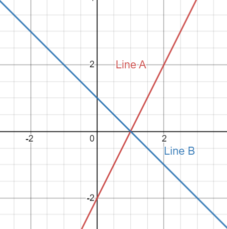
The first case is obvious, two lines intersect at one point. In this case, we have exactly one solution.
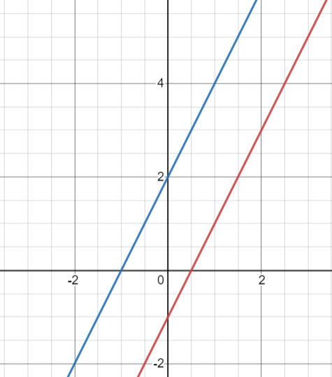
The second case is two parallel lines. In this case, we have zero solution.
The third case is less obvious, you can place your two lines at the same place. In this case, all the points on these lines are the solution. We can say there are infinite solutions.
I personally don’t like to say there are infinite many solutions. Here is the reason: Saying infinite solutions is not useful, at least in some cases. For example, there are infinitely many points on one line, but there are also infinite many points on two lines, a plane, a little triangle, or a cube. So only saying “there are infinitely many solutions” won’t give you enough information.
If we write these three different cases in augment matrix, you will see that the second one and the third one are very special:
Both cases has two linearly dependent rows, but the vectors on the right are different. Let’s look at them one by one:
This one is saying that \(2x-y = 2\) and also \(2x-y = -1\). Obviously, this will end up with no solution since you can combine them and give you \(2 = -1\). For this type of linear system, we say they are inconsistent.
Then let’s look at the next one:
This one is ridiculous. The two equations are literally the same thing! So it didn’t tell us enough information about the system! Of course you are getting infinite many solutions because you have two variables with only one equation.
So Let’s sum up here. If the matrix has linear dependent rows, then it means that at least one of the rows is “useless”. So if you have a \(n\times n\) matrix and one of the rows is telling the same thing as other rows, then you will not have sufficient conditions to solve this system. Then you will end up with many solutions.
If your matrix has linear dependent rows and the vector doesn’t match, then it means you have parallel lines&planes. Then you end up with no solution.
Then finally, if all your rows are linear independent, congratulation! You can have a non-trivial solution.
But why linear independent rows can give you non-trivial solutions? Let’s see if we can understand it using the knowledge of linear transformation.
The equation we are going to solve is this:
Solving this equation means to find the vector \(\pmb{\color{red}x}\) such that after the transformation it became \(\pmb{b}\).
By looking at the transformation, we can predict what will happen if we put a vector in there. Let’s start with a linear dependent matrix:
So what is the transformation looks like?
As you can see, all the vectors are transformed onto a line \(y = x\). This makes sense since the transformation returns exactly the same number for x and y. In fact, any linear dependent 2 by 2 matrix will squish the 2d plane to a line(or a point if everything is zero). So, if we are looking for a specific \(\pmb{\color{red}x}\) that gives you \(\pmb{b}\). Then there are two possible results: One is that your \(\pmb{b}\) actually landed on this line so you get some solution. The other case is your \(\pmb{b}\) is unfortunately not on this line so the system is inconsistent, no such \(\pmb{\color{red}x}\) can give you that \(\pmb{b}\) vector after the transformation.
Now, why do you have multiple solutions for one \(\pmb{b}\)? Well, If we just look at the transformation itself, it looks like all the vectors in 2d space are projected on the 1d line. Like the shadow under sun. So it kind of makes sense if different objects return exactly the same shadow.
But this is only 2 dimension. What if we have more than 2? what if we have the dimension of 10? how do we understand the transformation that happens in 100 dimensions? Obviously, we need more tools to do that. So, let’s use the knowledge of span and basis vector!
We know that we can think of any matrices as linear transformations, and each column in a transformation matrix tells us how basis vector transform. So why don’t we find the span of those basis vectors after the transformation? That will definitely give us some information about this transformation.
Let’s take the above matrix as a example:
The column vectors are:
So the span of those vectors gives us the \(y = x\) line on a 2d plane.
What do we know from this? We know that any vectors after this transformation will end up sitting on the line \(y = x\). Why? Well any vector on the plane can be rewrite into a linear combination of the basis vector:
Then if we apply the transformation:
So the vector after the transformation will be a linear combination of the column vectors \(T
Do that span of column vectors has a name? Yes, it is called Column space. By looking at the column space, we will know where our vectors live after the transformation. It is just like the idea of the range in function.
Let’s look at the dimension of column space. For a \(n \times n\) matrix, which means you have n variable and n equations(or you can think of a dimension n vector transform to a same dimension vector). We can say the dimension of the matrix is n. if its column space also has the dimension of n, what does this tell us? Well, it means your vector after the transformation lives in the same dimension n space. In other word, the columns are linearly independent. Later on, we will know that this also means the rows are linearly independent too.
Here is the tricky part. What if the dimension is less than n? You might say: Sure! Then it means the linear system has no solution or many solutions. But I want to know more about it.
An interesting question to ask is: We start with the dimension of n, we ended up with the dimension of something less than n, so where does this “missing” dimension go? Let’s look at the equation again:
Assume we have linearly independent columns (or you can say we have only one solution). Let’s call the solution \(\pmb{x}_1\), so:
Now let’s consider the similar equation:
if there is some non-zero \(\pmb{x}\) satisfy this equation, we are in big trouble. Why?
Assume that \(A\pmb{x}_2 = \pmb{0}\) for some non-zero \(\pmb{x}_2\), the I can say there exist a brand new solution for \(A\pmb{x} = \pmb{b}\):
The new solution is \(\pmb{x}_1 + \pmb{x}_2\). For linear independent matrix, this $\pmb{x}_2 $ has to be zero, otherwise you won’t get only one solution.
What if the rows are linear dependent? Then the equation \(A\pmb{x} = \pmb{0}\) will have non-zero solution!
Take the same matrix as example, if we solve \(A\pmb{x} = \pmb{0}\) for this matrix we will have:
This equation is easy to solve, we just have :
All the vectors on the line $ y = 2x $ satisify the equations. We can also write the result as:
We actually have a name for this space, we call it null space or Kernel. “Null” means “nothing”, Of course, this does not mean there is nothing in the space. It means the collection of all vectors that are transformed to “nothing”, the zero vector.
Let’s take a look at what null space is. Here I graphed a vector in 2d and drew some other vectors that are the linear combination of the null space vector and the original vector. Notice in our case, all such vector sits on a line since our null space is one dimensional.
As you can see, all the vectors were transformed into one same vector as we expected. if we know one solution of the linear system, adding any null space vector to that solution will give you a new solution. So if the null space of your matrix is not zero, then once you have a solution(if the system is consistent), you can get infinite many solutions from adding the null space vectors. But if the null space of your matrix is zero, you will just get a unique one.
By checking the column space and the null space of a linear system, it is fairly easy to tell if the system has solutions or not. Notice that we are no longer focusing on a single linear system. We are now treating the matrix as a linear transformation and focusing on how the whole space change. The linear equations only describe one result of this linear transformation. Once you understand this, it is much easier for you to understand why people are interested in linear algebra.